
You are given an array prices where prices[i] is the price of a given stock on the ith day.
You want to maximize your profit by choosing a single day to buy one stock and choosing a different day in the future to sell that stock.
Return the maximum profit you can achieve from this transaction. If you cannot achieve any profit, return 0.
Here’s the [Problem Link] to begin with.
Example 1:
Input: prices = [7,1,5,3,6,4]
Output: 5
Explanation: Buy on day 2 (price = 1) and sell on day 5 (price = 6), profit = 6-1 = 5.
Note that buying on day 2 and selling on day 1 is not allowed because you must buy before you sell.
Example 2:
Input: prices = [7,6,4,3,1]
Output: 0
Explanation: In this case, no transactions are done and the max profit = 0.
Constraints:
- 1 <= prices.length <= 105
- 0 <= prices[i] <= 104
BRUTE FORCE SOLUTION
1. Understanding the Problem
Objective:
Given an integer array prices, where prices[i] represents the price of a given stock on the ithi^{th}ith day, you aim to maximize your profit by choosing exactly one day to buy one stock and choosing a different day in the future to sell that stock. Return the maximum profit you can achieve from this transaction. If you cannot achieve any profit, return 0.
Problem Statement (LeetCode Reference):
You are given an array prices where prices[i] is the price of a given stock on the ithi^{th}ith day.
You want to maximize your profit by choosing a single day to buy one stock and choosing a different day in the future to sell that stock.
Return the maximum profit you can achieve from this transaction. If you cannot achieve any profit, return 0.
Example:
- Input:
prices = [7,1,5,3,6,4] - Output:
5 - Explanation:
Buy on day 2 (price = 1) and sell on day 5 (price = 6), profit = 6 – 1 = 5. Not 7-1 = 6, as selling price needs to be larger than buying price and days must follow.
2. Grasping the Strategy: Brute-Force Approach
The provided maxProfit function employs a brute-force approach to solve the problem. Here’s a high-level overview of the strategy:
- Iterate Through All Possible Pairs of Days:
- Use two nested loops to consider every possible pair of days where the first day (iii) is the buying day and the second day (jjj) is the selling day.
- The outer loop (for i in range(n)) selects the buying day.
- The inner loop (for j in range(i + 1, n)) selects the selling day, ensuring that the selling day is after the buying day.
- Calculate the Profit for Each Valid Pair:
- For each pair (i,j)(i, j)(i,j), check if the selling price (prices[j]) is higher than the buying price (prices[i]).
- If so, calculate the profit (prices[j] – prices[i]).
- Track the Maximum Profit:
- Compare the calculated profit with the current maximum profit (maxPro).
- Update maxPro if the new profit is greater.
- Return the Maximum Profit:
- After examining all possible pairs, return maxPro, which holds the largest profit found. If no profit is possible, maxPro remains 0.
Visualization:
Imagine you’re at a stock market, and you have the opportunity to buy and sell a stock. For each day, you decide whether to buy the stock on that day and then consider selling it on any future day to maximize your profit.
Analogy:
Think of the array as a timeline of stock prices. Your goal is to find the lowest point to buy and the highest point after that to sell, ensuring that the selling day comes after the buying day.
3. Code
class Solution:
def maxProfit(self, prices: List[int]) -> int:
maxPro = 0
n = len(prices)
for i in range(n):
for j in range(i + 1, n):
if prices[j] > prices[i]:
maxPro = max(prices[j] - prices[i], maxPro)
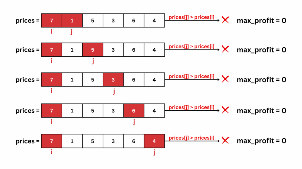
return maxPro4. Dry Run
Let’s go through the code step by step, using images to illustrate the detailed dry run process.

5. Time and Space Complexity
Time Complexity: O(n2)
- Explanation:
- Outer Loop (for i in range(n)):
Iterates n times, where n is the length of the prices array. - Inner Loop (for j in range(i + 1, n)):
For each i, iterates approximately n – i – 1 times. - Overall:
The combination of two nested loops results in a quadratic time complexity, O(n2), meaning that the execution time grows proportionally to the square of the input size. This approach is inefficient for large datasets.
- Outer Loop (for i in range(n)):
Space Complexity: O(1)
- Explanation:
- Variables Used:
- maxPro: Stores the maximum profit found so far.
- n: Stores the length of the prices array.
- Space Utilization:
The function uses a constant amount of additional space, regardless of the input size. No extra data structures (like arrays or hash maps) are used that scale with the input. - Overall:
The space complexity is constant, O(1), making the function space-efficient.
- Variables Used:
Efficiency Note:
While the brute-force approach correctly identifies the maximum profit by examining all possible pairs of days, its quadratic time complexity makes it impractical for large input sizes. For example, an array of size 10^5 would result in approximately 1010 operations, leading to significant performance delays.
OPTIMAL SOLUTION
1. Understanding the Problem
Objective:
Given an integer array prices, where prices[i] represents the price of a given stock on the ith day, you aim to maximize your profit by choosing exactly one day to buy one stock and choosing a different day in the future to sell that stock. Return the maximum profit you can achieve from this transaction. If you cannot achieve any profit, return 0.
Problem Statement (LeetCode Reference):
You are given an array prices where prices[i] is the price of a given stock on the ith day.
You want to maximize your profit by choosing a single day to buy one stock and choosing a different day in the future to sell that stock.
Return the maximum profit you can achieve from this transaction. If you cannot achieve any profit, return 0.
Example:
- Input:
prices = [7,1,5,3,6,4] - Output:
5 - Explanation:
Buy on day 2 (price = 1) and sell on day 5 (price = 6), profit = 6 – 1 = 5.
2. Grasping the Strategy: Optimized Linear Approach
The provided maxProfit function employs an optimized linear approach to solve the problem with linear time complexity. Here’s a high-level overview of the strategy:
- Initialization:
- max_profit = 0:
Initialize the maximum profit to 0. This variable will keep track of the highest profit found. - min_price = float(“inf”):
Initialize min_price to positive infinity. This variable will track the lowest price encountered so far.
- max_profit = 0:
- Iterate Through the Array:
- Loop (for i in range(len(prices))):
Traverse each element in the array using its index i. - Update Minimum Price (min_price):
At each step, update min_price to be the minimum of the current min_price and prices[i]. This ensures that min_price always holds the lowest price up to the current day. - Calculate Potential Profit and Update Maximum Profit (max_profit):
Calculate the potential profit by subtracting the current min_price from prices[i] (i.e., prices[i] – min_price). Update max_profit if this potential profit is greater than the current max_profit.
- Loop (for i in range(len(prices))):
- Return the Result:
- After traversing the entire array, return the value of max_profit, which holds the largest profit found. If no profit is possible, max_profit remains 0.
Visualization:
Imagine you’re at a stock market, and you’re tracking the lowest price you’ve seen so far. As you move through each day’s price, you calculate the profit you’d make if you sold on that day by subtracting the lowest price from the current price. You keep updating your maximum profit as you find better opportunities.
Analogy:
Think of the array as a timeline of stock prices. Your goal is to find the lowest valley (minimum price) and the highest peak (maximum price after the valley) to maximize your elevation gain (profit), ensuring that the peak comes after the valley.
3. Code
class Solution:
    def maxProfit(self, prices: List[int]) -> int:
        max_profit = 0
        min_price = float("inf")
        for i in range(len(prices)):
            min_price = min(min_price, prices[i])
            max_profit = max(max_profit, prices[i] - min_price)
        return max_profit
Let’s walk through how the maxProfit function operates using an illustrative example.
Example:
- Input:
prices = [7,1,5,3,6,4] - Execution Steps:
- Initialization:
- max_profit = 0
- min_price = float(“inf”)
- Iteration Through the Array:
- Initialization:
| Day (i) | Price (prices[i]) | min_price Calculation | max_profit Calculation | max_profit Update |
| 0 | 7 | min_price = min(inf, 7) = 7 | profit = 7 – 7 = 0 | max_profit = max(0, 0) = 0 |
| 1 | 1 | min_price = min(7, 1) = 1 | profit = 1 – 1 = 0 | max_profit = max(0, 0) = 0 |
| 2 | 5 | min_price = min(1, 5) = 1 | profit = 5 – 1 = 4 | max_profit = max(0, 4) = 4 |
| 3 | 3 | min_price = min(1, 3) = 1 | profit = 3 – 1 = 2 | max_profit = max(4, 2) = 4 |
| 4 | 6 | min_price = min(1, 6) = 1 | profit = 6 – 1 = 5 | max_profit = max(4, 5) = 5 |
| 5 | 4 | min_price = min(1, 4) = 1 | profit = 4 – 1 = 3 | max_profit = max(5, 3) = 5 |
- Final Result:
- After traversing the entire array, the maximum profit found is 5, achieved by buying on day 1 (price = 1) and selling on day 4 (price = 6).
- Return:
- The function returns 5.
4. Visualizing the Process
To better comprehend how the optimized linear approach works, let’s visualize the traversal and the state of the variables at each step.
Array: [7, 1, 5, 3, 6, 4]
Index: 0 1 2 3 4 5
- Initial State:
- max_profit = 0
- min_price = ∞
- Steps:
- Day 0 (Price = 7):
- min_price = min(∞, 7) = 7
- profit = 7 – 7 = 0
- max_profit = max(0, 0) = 0
- Day 1 (Price = 1):
- min_price = min(7, 1) = 1
- profit = 1 – 1 = 0
- max_profit = max(0, 0) = 0
- Day 2 (Price = 5):
- min_price = min(1, 5) = 1
- profit = 5 – 1 = 4
- max_profit = max(0, 4) = 4
- Day 3 (Price = 3):
- min_price = min(1, 3) = 1
- profit = 3 – 1 = 2
- max_profit = max(4, 2) = 4
- Day 4 (Price = 6):
- min_price = min(1, 6) = 1
- profit = 6 – 1 = 5
- max_profit = max(4, 5) = 5
- Day 5 (Price = 4):
- min_price = min(1, 4) = 1
- profit = 4 – 1 = 3
- max_profit = max(5, 3) = 5
- Day 0 (Price = 7):
- Final State:
- max_profit = 5
- The subarray contributing to max_profit is buying on day 1 and selling on day 4.
5. Time and Space Complexity
Time Complexity: O(n)
- Explanation:
- Single Pass Traversal:
The function iterates through the array prices once, performing constant-time operations at each step. - Loop Operations:
- Finding Minimum Price (min_price = min(min_price, prices[i])):
Takes constant time. - Calculating and Updating Maximum Profit (max_profit = max(max_profit, prices[i] – min_price)):
Takes constant time.
- Finding Minimum Price (min_price = min(min_price, prices[i])):
- Overall:
Since all operations within the loop are constant time and the loop runs n times (where n is the length of prices), the total time complexity is linear, O(n).
- Single Pass Traversal:
Space Complexity: O(1)
- Explanation:
- Variables Used:
- max_profit: Stores the maximum profit found so far.
- min_price: Stores the minimum price encountered so far.
- n: Stores the length of the prices array.
- Space Utilization:
The function uses a constant amount of additional space, regardless of the input size. No extra data structures (like arrays or hash maps) are used that scale with the input. - Overall:
The space complexity is constant, O(1), making the function space-efficient.
- Variables Used:
Efficiency Note:
This optimized linear approach is highly efficient for the Best Time to Buy and Sell Stock problem due to its linear time and constant space complexities. It ensures that even for large datasets, the function performs optimally without unnecessary computational overhead.
For any changes to the article, kindly email at code@codeanddebug.in or contact us at +91-9712928220.