

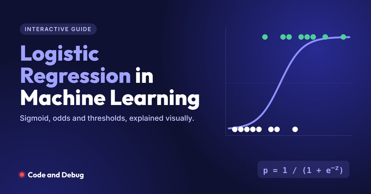
Is this email spam? Will this customer repay the loan? Does this scan show a tumour? Will a student pass the exam? Questions with a yes or no answer are everywhere, and logistic regression is the first algorithm most data scientists reach for to answer them.
This guide explains logistic regression in machine learning from the ground up, with something to play with in every section. You will bend the sigmoid curve yourself, convert probabilities into odds, draw a decision boundary by adding points, tune a spam filter’s threshold, and watch the model train. If you have not read our linear regression guide yet, it helps, but it is not required.
What is logistic regression in machine learning?
Logistic regression is a supervised machine learning algorithm used for classification. It looks at the input features, calculates the probability that an example belongs to a class, and then picks the class based on that probability. For a student who studied 6 hours, it might say “82% chance of passing”, and since 82% is above 50%, it predicts pass.
Some everyday uses:
- Spam detection: spam or not spam
- Credit risk: will a borrower default or repay
- Medical diagnosis: is a tumour malignant or benign
- Marketing: will a user click the ad or buy the product
- HR analytics: will an employee leave in the next year
Is logistic regression classification or regression?
Classification. The final output is a class label, like pass or fail. Under the hood, though, it does predict a number, the probability of the class, and the probability is what makes it so useful: you know how sure the model is, not only what it chose.
Why is it called regression?
Because the core of the model is a linear regression. It computes a weighted sum of the features, exactly like linear regression does, and then passes that sum through the logistic (sigmoid) function to turn it into a probability. Statisticians named it after that structure long before machine learning existed, and the name stuck.
The sigmoid function
A plain straight line can produce any number, like 1.44 or −0.3, which makes no sense as a probability. The sigmoid function, also called the logistic function, fixes that by squashing any number into the range 0 to 1:
When z is a large positive number, σ(z) gets close to 1. When z is very negative, it gets close to 0. When z is exactly 0, the output is exactly 0.5. Plotted on a graph, it makes the famous S-shaped curve.
Below, the dots are 16 students: green passed, dark failed. Move the weight and bias to fit the S-curve to the data. The weight controls how steep the curve is, and the bias slides it left or right. Your goal is the lowest log loss, which we explain later.
Fit the sigmoid curve yourself
Hours studied vs passing the exam.
Logistic regression formula and equation
With one feature, the logistic regression model is:
With many features, the weighted sum simply gets longer:
Here p is the probability of the positive class (pass, spam, default), the b values are the coefficients the model learns, and the x values are your features.
Odds, log-odds and the logit
There is a second way to write the same model that explains what the coefficients mean. First, odds compare the chance of something happening to the chance of it not happening:
The second line is the key insight: logistic regression is a linear model for the log-odds. The log-odds function is also called the logit. Drag the slider to see how the three quantities relate.
Probability, odds and log-odds converter
Each dot is one student out of 20 similar students.
This is how you read a coefficient: increasing a feature by 1 adds its coefficient to the log-odds, which multiplies the odds by ecoefficient. This number is called the odds ratio. In our Python example below the model learns w = 0.892 for hours studied, and e0.892 ≈ 2.44. So every extra hour of study multiplies a student’s odds of passing by about 2.4.
Decision boundary
Once the model outputs a probability, it needs a rule to choose a class. The default rule is simple: predict 1 if p ≥ 0.5, otherwise predict 0. Since p = 0.5 exactly when the weighted sum is 0, the dividing line between the classes is where b₀ + b₁x₁ + b₂x₂ = 0. With two features that is a straight line, called the decision boundary.
Below, each dot is a student described by two features: hours studied and attendance. The model is trained live in your browser. Click on the chart to add a student and watch it retrain and the boundary move. Ringed dots are students the model gets wrong.
Draw the decision boundary
Pick a class, then click on the chart to add students.
Notice that the boundary is always a straight line. That is why logistic regression is called a linear classifier. If the real boundary between classes is curved, you need extra features, like squares of the inputs, or a different model.
Choosing the threshold: precision vs recall
A threshold of 0.5 is only a default. In real projects you choose it based on which mistake costs more. Missing a cancer case is far worse than a false alarm, so a screening model uses a low threshold. A spam filter that sends your job offer to spam is worse than letting one spam email through, so it uses a high threshold.
Below are 20 emails with the spam probability a logistic regression model gave each one. Move the threshold and watch the four outcomes change. This 2 × 2 table is called a confusion matrix.
Tune a spam filter
Red dots are real spam, green dots are genuine emails.
Cost function: log loss
Linear regression measures error with mean squared error. Logistic regression cannot, because squared error combined with the sigmoid creates a bumpy error surface with many local minimums, and gradient descent can get stuck. Instead it uses log loss, also called binary cross-entropy:
It looks complicated, but only one half is active for each example. If the true label is 1, the penalty is −ln(p). If the true label is 0, it is −ln(1 − p). Try it below and compare it with squared error, shown as the dashed line.
How log loss punishes mistakes
Choose the true label, then change the model’s prediction.
Being confident and wrong is extremely expensive under log loss. That pressure is exactly what pushes the model towards honest, well-calibrated probabilities.
How logistic regression learns: maximum likelihood and gradient descent
Training means finding the weights that make the observed data most likely. This idea is called maximum likelihood estimation (MLE), and minimising log loss is the same thing as maximising likelihood. There is no neat formula for the answer like there is for linear regression, so the weights are found step by step with gradient descent. The update rule is surprisingly simple:
Press Run and watch a flat 50% line bend into the S-curve as the log loss falls.
Watch logistic regression train
Left: the model’s curve. Right: log loss falling over time.
Types of logistic regression
- Binary logistic regression: two classes, like spam or not spam. This is what most of this guide covers.
- Multinomial logistic regression: three or more classes with no natural order, like classifying news into sports, politics or tech. It is also called nominal or softmax regression.
- Ordinal logistic regression: three or more classes that do have an order, like movie ratings from 1 to 5 or survey answers from “disagree” to “agree”.
Multinomial logistic regression computes one score per class and uses the softmax function to turn the scores into probabilities that add up to 1. Here a model is predicting which course track a student will choose:
Softmax: from scores to probabilities
Change each class’s score and watch the probabilities rebalance.
Assumptions of logistic regression
Logistic regression needs fewer assumptions than linear regression. It does not need normally distributed errors or equal variance. It does need these:
- The right kind of target: binary for binary logistic regression, categories for multinomial, ordered categories for ordinal.
- Independent observations: one row should not influence another, so no repeated measurements of the same person treated as separate people.
- Little multicollinearity: features should not be strongly correlated with each other, or the coefficients become unstable.
- Linear relationship with the log-odds: each continuous feature should relate roughly linearly to the log-odds of the outcome.
- Enough data: a common rule of thumb is at least 10 examples of the rarer class for every feature.
- No extreme outliers in the features, since they can pull the boundary off course.
Linear regression vs logistic regression
These two get compared all the time because their names and formulas look so similar. Our linear regression guide has a demo showing a straight line predicting a 144% chance of passing, which is exactly the problem logistic regression solves. Here is the full comparison:
| Linear regression | Logistic regression | |
|---|---|---|
| Problem type | Regression | Classification |
| Output | Any real number | Probability between 0 and 1, then a class |
| Curve | Straight line | S-shaped sigmoid |
| Core equation | y = b₀ + b₁x₁ + … + bₙxₙ | log-odds = b₀ + b₁x₁ + … + bₙxₙ |
| Loss function | Mean squared error | Log loss (cross-entropy) |
| How it is solved | Exact formula or gradient descent | Gradient descent (maximum likelihood) |
| Evaluation | MAE, RMSE, R² | Accuracy, precision, recall, F1, ROC-AUC |
| Example | Predict a flat’s price | Predict if a loan will default |
Logistic regression in Python with scikit-learn
You need NumPy and scikit-learn (pip install numpy scikit-learn). Every output below comes from actually running the code.
Simple example: will the student pass?
import numpy as np
from sklearn.linear_model import LogisticRegression

# Hours studied and whether the student passed (1) or failed (0)
hours = np.array([0.5, 1, 1.5, 2, 2.5, 3, 3.5, 4, 4.5, 5,
                  5.5, 6, 6.5, 7, 8, 9.5]).reshape(-1, 1)
passed = np.array([0, 0, 0, 0, 0, 1, 0, 0, 1, 1, 0, 1, 1, 1, 1, 1])

model = LogisticRegression()
model.fit(hours, passed)

print("Weight (w):", round(model.coef_[0][0], 3))
print("Bias (b):", round(model.intercept_[0], 3))

for h in [2, 4.5, 7]:
    p = model.predict_proba([[h]])[0][1]
    print(f"{h} hours -> {p:.0%} chance of passing -> predicted class {model.predict([[h]])[0]}")
Output:
Weight (w): 0.892
Bias (b): -3.814
2 hours -> 12% chance of passing -> predicted class 0
4.5 hours -> 55% chance of passing -> predicted class 1
7 hours -> 92% chance of passing -> predicted class 1
predict_proba gives the probability of each class, and predict applies the 0.5 threshold for you. To use a different threshold, take the probabilities and compare them yourself, for example (model.predict_proba(X)[:, 1] >= 0.3).
Real dataset: breast cancer classification
scikit-learn ships with a real medical dataset of 569 tumours, each described by 30 measurements. Scaling the features first helps the solver converge.
from sklearn.datasets import load_breast_cancer
from sklearn.model_selection import train_test_split
from sklearn.pipeline import make_pipeline
from sklearn.preprocessing import StandardScaler
from sklearn.linear_model import LogisticRegression
from sklearn.metrics import accuracy_score, confusion_matrix, classification_report

# 569 tumour samples, 30 measurements each. Target: 0 = malignant, 1 = benign
X, y = load_breast_cancer(return_X_y=True)
X_train, X_test, y_train, y_test = train_test_split(
    X, y, test_size=0.2, random_state=42, stratify=y)

# Scale the features, then fit logistic regression
model = make_pipeline(StandardScaler(), LogisticRegression(max_iter=1000))
model.fit(X_train, y_train)
pred = model.predict(X_test)

print("Accuracy:", round(accuracy_score(y_test, pred), 3))
print("Confusion matrix:")
print(confusion_matrix(y_test, pred))
print(classification_report(y_test, pred, target_names=["malignant", "benign"]))
Output:
Accuracy: 0.982
Confusion matrix:
[[41  1]
 [ 1 71]]
              precision    recall  f1-score   support

   malignant       0.98      0.98      0.98        42
      benign       0.99      0.99      0.99        72

    accuracy                           0.98       114
   macro avg       0.98      0.98      0.98       114
weighted avg       0.98      0.98      0.98       114
The model gets 98% of the test tumours right, misclassifying only 2 out of 114. In the confusion matrix, rows are the true classes and columns are the predicted ones, so the top-right 1 is a malignant tumour predicted as benign. In a real medical project that is the most dangerous mistake, and you would lower the threshold to push it towards zero.
Logistic regression from scratch with NumPy
This is the same gradient descent you watched in the training demo:
import numpy as np

x = np.array([0.5, 1, 1.5, 2, 2.5, 3, 3.5, 4, 4.5, 5,
              5.5, 6, 6.5, 7, 8, 9.5])
y = np.array([0, 0, 0, 0, 0, 1, 0, 0, 1, 1, 0, 1, 1, 1, 1, 1])

def sigmoid(z):
    return 1 / (1 + np.exp(-z))

w, b = 0.0, 0.0
lr = 0.1

for step in range(20000):
    p = sigmoid(w * x + b)          # predicted probabilities
    dw = np.mean((p - y) * x)       # gradient of log loss for w
    db = np.mean(p - y)             # gradient of log loss for b
    w -= lr * dw
    b -= lr * db

loss = -np.mean(y * np.log(p) + (1 - y) * np.log(1 - p))
print("w =", round(w, 3), " b =", round(b, 3), " log loss =", round(loss, 3))
print("Hours needed for a 50% chance:", round(-b / w, 2))
Output:
w = 1.087  b = -4.632  log loss = 0.353
Hours needed for a 50% chance: 4.26
The weights differ from the scikit-learn example (1.087 here vs 0.892 there) because scikit-learn adds L2 regularisation by default (the C=1.0 parameter), which gently shrinks weights to reduce overfitting. Set LogisticRegression(C=1e9) to switch it off and you get 1.087 and −4.633, exactly matching the NumPy version.
Advantages and limitations
- Gives probabilities, not just labels, so you can set your own threshold and rank cases by risk.
- Easy to interpret. Each coefficient converts into an odds ratio that a manager or doctor can understand.
- Fast and light. It trains in seconds on millions of rows and is a strong baseline for any classification problem.
- Only draws straight boundaries unless you engineer extra features.
- Struggles with highly correlated features and needs care with imbalanced classes, for example using
class_weight="balanced".
Test yourself
Six questions. Five or more correct and you are ready to use logistic regression on a real problem.
Logistic regression quiz
Takes about two minutes.
Frequently asked questions
Is logistic regression supervised or unsupervised learning?
Supervised. It learns from examples where the correct class is already known, such as emails already labelled as spam or not spam.
Is logistic regression a classification or regression algorithm?
It is a classification algorithm. It predicts the probability of a class and then assigns the class using a threshold, usually 0.5.
Why is logistic regression called regression if it does classification?
Because its core is a linear regression on the log-odds of the outcome. The logistic (sigmoid) function then converts that value into a probability. The name comes from statistics and predates its use as a classifier.
What is the sigmoid function in logistic regression?
The sigmoid function σ(z) = 1 / (1 + e^−z) maps any real number to a value between 0 and 1. Logistic regression applies it to the weighted sum of features so the output can be read as a probability.
What is the cost function of logistic regression?
Log loss, also called binary cross-entropy: −(1/n) Σ [y ln(p) + (1 − y) ln(1 − p)]. It heavily penalises confident wrong predictions and gives a convex error surface that gradient descent can minimise reliably.
What is the difference between linear and logistic regression?
Linear regression predicts a continuous number with a straight line and minimises squared error. Logistic regression predicts the probability of a class with an S-shaped sigmoid curve and minimises log loss.
Can logistic regression handle more than two classes?
Yes. Multinomial logistic regression uses the softmax function to handle three or more unordered classes, and ordinal logistic regression handles ordered classes such as ratings.
What to learn next
You now know how to build a classifier and why the threshold matters. The natural next topics are the confusion matrix and its metrics in more depth, then decision trees and random forests, which can draw curved boundaries. Our interactive AI and ML roadmap shows where each of these fits, and the linear regression guide covers the regression side.
